
Forecast prediction is predicting a future value using past values and many other factors. In this tutorial, we will create a sales forecasting model using the Keras functional API.
Sales forecasting
It is determining present-day or future sales using data like past sales, seasonality, festivities, economic conditions, etc.
So, this model will predict sales on a certain day after being provided with a certain set of inputs.
In this model 8 parameters were used as input:
- past seven day sales
- day of the week
- date – the date was transformed into 3 different inputs
- season
- Festival or not
- sales on the same day in the previous year
How does it work?
First, all inputs are preprocessed to be understandable by the machine. This is a linear regression model based on supervised learning, so the output will be provided along with the input. Then inputs are then fed to the model along with desired output. The model will plot(learn) a relation(function) between the input and output. This function or relation is then used to predict the output for a specific set of inputs. In this case, input parameters like date and previous sales are labeled as input, and the amount of sales is marked as output. The model will predict a number between 0 and 1 as a sigmoid function is used in the last layer. This output can be multiplied by a specific number(in this case, maximum sales), this will be our corresponding sales amount for a certain day. This output is then provided as input to calculate sales data for the next day. This cycle of steps will be continued until a certain date arrives.
Required packages and Installation
- numpy
- pandas
- keras
- tensorflow
- csv
- matplotlib.pyplot
import pandas as pd # to extract data from dataset(.csv file)
import csv #used to read and write to csv files
import numpy as np #used to convert input into numpy arrays to be fed to the model
import matplotlib.pyplot as plt #to plot/visualize sales data and sales forecasting
import tensorflow as tf # acts as the framework upon which this model is built
from tensorflow import keras #defines layers and functions in the model
#here the csv file has been copied into three lists to allow better availability
list_row,date,traffic = get_data('/home/abh/Documents/Python/Untitled Folder/Sales_dataset')
The use of external libraries has been kept to a minimum to provide a simpler interface, you can replace the functions used in this tutorial with those already existing in established libraries.
Original data set for sales data for 5 years:
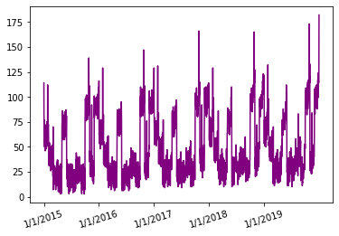
Sales data from Jan 2015 to Dec 2019
As you can see, the sales data seems to be following a similar kind of pattern for each year and the peak sales value seems to be increasing with time over the 5-year time frame.
In this 5-year time frame, the first 4 years will be used to train the model and the last year will be used as a test set.
Now, a few helper functions were used for processing the dataset and creating inputs of the required shape and size. They are as follows:
- get_data – used to load the data set using a path to its location.
- date_to_day – provides a day to each day. For example — 2/2/16 is Saturday and 9/5/15 is Monday.
- date_to_enc – Encodes data into one-hot vectors, this provides a better learning opportunity for the model.
All the properties of these functions and a few other functions cannot be explained here as it would take too much time. Please visit this link if you want to look at the entire code.
Preprocessing:
Initially, the data set had only two columns: date and traffic(sales).
After the addition of different columns and processing/normalization of values, the data contained all these values.
- Date
- Traffic
- Holiday or not
- Day
All these parameters have to be converted into a form that the machine can understand, which will be done using this function below.
Instead of keeping date, month, and year as a single entity, it was broken into three different inputs. The reason is that the year parameter in these inputs will be the same most of the time, this will cause the model to become complacent i.e it will begin to overfit to the current dataset. To increase the variability between different various inputs dates, days and months were labeled separately. The following function conversion() will create six lists and append appropriate input to them. This is how years 2015 to 2019 will look as an encoding: is
{2015: array([1., 0., 0., 0., 0.], dtype=float32), 2016: array([0., 1., 0., 0., 0.], dtype=float32), 2017: array([0., 0., 1., 0., 0.], dtype=float32), 2018: array([0., 0., 0., 1., 0.], dtype=float32), 2019: array([0., 0., 0., 0., 1.], dtype=float32)
Each of them is a NumPy array of length 5 with 1s and 0s denoting its value
def conversion(week,days,months,years,list_row):
#lists have been defined to hold different inputs
inp_day = []
inp_mon = []
inp_year = []
inp_week=[]
inp_hol=[]
out = []
#converts the days of a week(monday,sunday,etc.) into one hot vectors and stores them as a dictionary
week1 = number_to_one_hot(week)
#list_row contains primary inputs
for row in list_row:
#Filter out date from list_row
d = row[0]
#the date was split into three values date, month and year.
d_split=d.split('/')
if d_split[2]==str(year_all[0]):
#prevents use of the first year data to ensure each input contains previous year data as well.
continue
#encode the three parameters of date into one hot vectors using date_to_enc function.
d1,m1,y1 = date_to_enc(d,days,months,years) #days, months and years and dictionaries containing the one hot encoding of each date,month and year.
inp_day.append(d1) #append date into date input
inp_mon.append(m1) #append month into month input
inp_year.append(y1) #append year into year input
week2 = week1[row[3]] #the day column from list_is converted into its one-hot representation and saved into week2 variable
inp_week.append(week2)# it is now appended into week input.
inp_hol.append([row[2]])#specifies whether the day is a holiday or not
t1 = row[1] #row[1] contains the traffic/sales value for a specific date
out.append(t1) #append t1(traffic value) into a list out
return inp_day,inp_mon,inp_year,inp_week,inp_hol,out #all the processed inputs are returned
inp_day,inp_mon,inp_year,inp_week,inp_hol,out = conversion(week,days,months,years,list_train)
#all of the inputs must be converted into numpy arrays to be fed into the model
inp_day = np.array(inp_day)
inp_mon = np.array(inp_mon)
inp_year = np.array(inp_year)
inp_week = np.array(inp_week)
inp_hol = np.array(inp_hol)
We will now process some other inputs that were remaining, the reason behind using all these parameters is to increase the efficiency of the model, you can experiment with removing or adding some inputs.
Sales data of the past seven days were passed as an input to create a trend in sales data, this will the predicted value will not be completely random similarly, sales data of the same day in the previous year was also provided.
The following function(other_inputs) processes three inputs:
- sales data of past seven days
- sales data on the same date in the previous year
- seasonality – seasonality was added to mark trends like summer sales, etc.
def other_inputs(season,list_row):
#lists to hold all the inputs
inp7=[]
inp_prev=[]
inp_sess=[]
count=0 #count variable will be used to keep track of the index of current row in order to access the traffic values of past seven days.
for row in list_row:
ind = count
count=count+1
d = row[0] #date was copied to variable d
d_split=d.split('/')
if d_split[2]==str(year_all[0]):
#preventing use of the first year in the data
continue
sess = cur_season(season,d) #assigning a season to the current date
inp_sess.append(sess) #appending sess variable to an input list
t7=[] #temporary list to hold seven sales value
t_prev=[] #temporary list to hold the previous year sales value
t_prev.append(list_row[ind-365][1]) #accessing the sales value from one year back and appending them
for j in range(0,7):
t7.append(list_row[ind-j-1][1]) #appending the last seven days sales value
inp7.append(t7)
inp_prev.append(t_prev)
return inp7,inp_prev,inp_sess
inp7,inp_prev,inp_sess = other_inputs(season,list_train)
inp7 = np.array(inp7)
inp7= inp7.reshape(inp7.shape[0],inp7.shape[1],1)
inp_prev = np.array(inp_prev)
inp_sess = np.array(inp_sess)
The reason behind so many inputs is that if all of these were combined into a single array, it would have different rows or columns of different lengths. Such an array cannot be fed as an input.
Linearly arranging all the values in a single array lead to the model having a high loss.
A linear arrangement will cause the model to generalize, as the difference between successive inputs would not be too different, which will lead to limited learning, decreasing the accuracy of the model.
Defining the Model
Eight separate inputs are processed and concatenated into a single layer and passed to the model.
The finalized inputs are as follows:
- Date
- Month
- Year
- Day
- Previous seven days sales
- sales in the previous year
- Season
- Holiday or not
Here in most layers, I have used 5 units as the output shape, you can further experiment with it to increase the efficiency of the model.
from tensorflow.keras.models import Model
from tensorflow.keras.layers import Input, Dense,LSTM,Flatten
from tensorflow.keras.layers import concatenate
#an Input variable is made from every input array
input_day = Input(shape=(inp_day.shape[1],),name = 'input_day')
input_mon = Input(shape=(inp_mon.shape[1],),name = 'input_mon')
input_year = Input(shape=(inp_year.shape[1],),name = 'input_year')
input_week = Input(shape=(inp_week.shape[1],),name = 'input_week')
input_hol = Input(shape=(inp_hol.shape[1],),name = 'input_hol')
input_day7 = Input(shape=(inp7.shape[1],inp7.shape[2]),name = 'input_day7')
input_day_prev = Input(shape=(inp_prev.shape[1],),name = 'input_day_prev')
input_day_sess = Input(shape=(inp_sess.shape[1],),name = 'input_day_sess')
# The model is quite straight-forward, all inputs were inserted into a dense layer with 5 units and 'relu' as activation function
x1 = Dense(5, activation='relu')(input_day)
x2 = Dense(5, activation='relu')(input_mon)
x3 = Dense(5, activation='relu')(input_year)
x4 = Dense(5, activation='relu')(input_week)
x5 = Dense(5, activation='relu')(input_hol)
x_6 = Dense(5, activation='relu')(input_day7)
x__6 = LSTM(5,return_sequences=True)(x_6) # LSTM is used to remember the importance of each day from the seven days data
x6 = Flatten()(x__10) # done to make the shape compatible to other inputs as LSTM outputs a three dimensional tensor
x7 = Dense(5, activation='relu')(input_day_prev)
x8 = Dense(5, activation='relu')(input_day_sess)
c = concatenate([x1,x2,x3,x4,x5,x6,x7,x8]) # all inputs are concatenated into one
layer1 = Dense(64,activation='relu')(c)
outputs = Dense(1, activation='sigmoid')(layer1) # a single output is produced with value ranging between 0-1.
# now the model is initialized and created as well
model = Model(inputs=[input_day,input_mon,input_year,input_week,input_hol,input_day7,input_day_prev,input_day_sess], outputs=outputs)
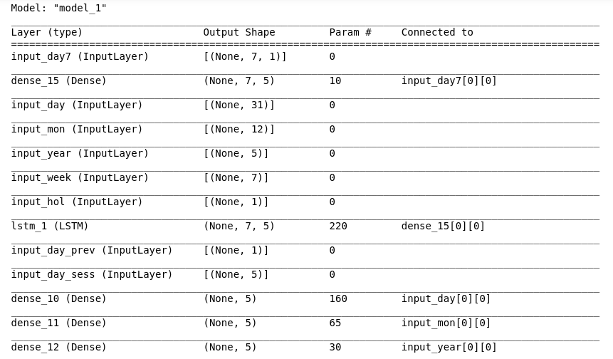
model.summary() # used to draw a summary(diagram) of the model
Model Summary:
Compiling the model using RMSprop:
RMSprop is great at dealing with random distributions, hence its use here.
from tensorflow.keras.optimizers import RMSprop
model.compile(loss=['mean_squared_error'],
optimizer = 'adam',
metrics = ['acc'] #while accuracy is used as a metrics here it will remain zero as this is no classification model
) # linear regression models are best gauged by their loss value
Fitting the model on the dataset:
The model will now be fed with the input and output data, this is the final step and now our model will be able to predict sales data.
history = model.fit(
x = [inp_day,inp_mon,inp_year,inp_week,inp_hol,inp7,inp_prev,inp_sess],
y = out,
batch_size=16,
steps_per_epoch=50,
epochs = 15,
verbose=1,
shuffle =False
)
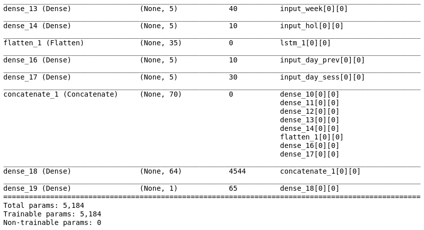
#all the inputs were fed into the model and the training was completed
Output:
Now, to test the model, input() takes input and transform it into the appropriate form:
def input(date):
d1,d2,d3 = date_to_enc(date,days,months,years) #separate date into three parameters
print('date=',date)
d1 = np.array([d1])
d2 = np.array([d2])
d3 = np.array([d3])
week1 = number_to_one_hot(week) #defining one hot vector to encode days of a week
week2 = week1[day[date]]
week2=np.array([week2])
//appeding a column for holiday(0-not holiday, 1- holiday)
if date in holiday:
h=1
#print('holiday')
else:
h=0
#print("no holiday")
h = np.array([h])
sess = cur_season(season,date) #getting seasonality data from cur_season function
sess = np.array([sess])
return d1,d2,d3,week2,h,sess
Predicting sales data is not what we are here for right, so let’s get on with the forecasting job.
Sales Forecasting
Defining forecast_testing function to forecast the sales data from one year back from provided date:
This function works as follows:
- A date is required as input to forecast the sales data from one year back till the mentioned date
- Then, we access the previous year’s sales data on the same day and sales data of 7 days before it.
- Then, using these as input a new value is predicted, then in the seven days value the first day is removed and the predicted output is added as input for the next prediction
For eg: we require forecasting of one year till 31/12/2019
- First, the date of 31/12/2018 (one year back) is recorded, and also seven-day sales from (25/12/2018 – 31/12/2018)
- Then the sales data of one year back i.e 31/12/2017 is collected
- Using these as inputs with other ones, the first sales data(i.e 1/1/2019) is predicted
- Then 24/12/2018 sales data is removed and 1/1/2019 predicted sales are added. This cycle is repeated until the sales data for 31/12/2019 is predicted.
So, previous outputs are used as inputs.
def forecast_testing(date):
maxj = max(traffic) # determines the maximum sales value in order to normalize or return the data to its original form
out=[]
count=-1
ind=0
for i in list_row:
count =count+1
if i[0]==date: #identify the index of the data in list
ind = count
t7=[]
t_prev=[]
t_prev.append(list_row[ind-365][1]) #previous year data
# for the first input, sales data of last seven days will be taken from training data
for j in range(0,7):
t7.append(list_row[ind-j-365][1])
result=[] # list to store the output and values
count=0
for i in list_date[ind-364:ind+2]:
d1,d2,d3,week2,h,sess = input(i) # using input function to process input values into numpy arrays
t_7 = np.array([t7]) # converting the data into a numpy array
t_7 = t_7.reshape(1,7,1)
# extracting and processing the previous year sales value
t_prev=[]
t_prev.append(list_row[ind-730+count][1])
t_prev = np.array([t_prev])
#predicting value for output
y_out = model.predict([d1,d2,d3,week2,h,t_7,t_prev,sess])
#output and multiply the max value to the output value to increase its range from 0-1
print(y_out[0][0]*maxj)
t7.pop(0) #delete the first value from the last seven days value
t7.append(y_out[0][0]) # append the output as input for the seven days data
result.append(y_out[0][0]*maxj) # append the output value to the result list
count=count+1
return result
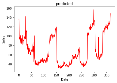
Run the forecast test function and a list containing all the sales data for that one year are returned
Result = forecast_testing(’31/12/2019′, date)
Graphs for both the forecast and actual values to test the performance of the model
plt.plot(result,color='red',label='predicted')
plt.plot(test_sales,color='purple',label="actual")
plt.xlabel("Date")
plt.ylabel("Sales")
leg = plt.legend()
plt.show()
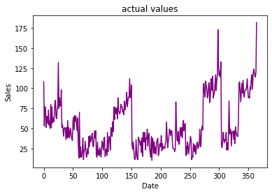
Actual Values from 1/1/2019 to 31/12/2019
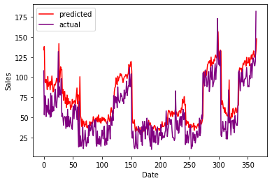
Comparison between prediction and actual values
As you can see, the predicted and actual values are quite close to each other, this proves the efficiency of our model. If there are any errors or possibilities of improvements in the above article, please feel free to mention them in the comment section.