
Dataset:
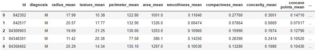
It is given by Kaggle from UCI Machine Learning Repository, in one of its challenge. It is a dataset of Breast Cancer patients with Malignant and Benign tumor.
Logistic Regression is used to predict whether the given patient is having Malignant or Benign tumor based on the attributes in the given dataset.
Code : Loading Libraries
# performing linear algebra
import numpy as np
# data processing
import pandas as pd
# visualisation
import matplotlib.pyplot as plt
Code : Loading dataset
data = pd.read_csv("..\breast-cancer-wisconsin-data\data.csv")
print (data.head)
Output :
Code : Loading dataset
data.info()
Output :
<class 'pandas.core.frame.DataFrame'>
RangeIndex: 569 entries, 0 to 568
Data columns (total 33 columns):
 #   Column                   Non-Null Count  Dtype
---  ------                   --------------  -----
 0   id                       569 non-null    int64
 1   diagnosis                569 non-null    object
 2   radius_mean              569 non-null    float64
 3   texture_mean             569 non-null    float64
 4   perimeter_mean           569 non-null    float64
 5   area_mean                569 non-null    float64
 6   smoothness_mean          569 non-null    float64
 7   compactness_mean         569 non-null    float64
 8   concavity_mean           569 non-null    float64
 9   concave points_mean      569 non-null    float64
 10  symmetry_mean            569 non-null    float64
 11  fractal_dimension_mean   569 non-null    float64
 12  radius_se                569 non-null    float64
 13  texture_se               569 non-null    float64
 14  perimeter_se             569 non-null    float64
 15  area_se                  569 non-null    float64
 16  smoothness_se            569 non-null    float64
 17  compactness_se           569 non-null    float64
 18  concavity_se             569 non-null    float64
 19  concave points_se        569 non-null    float64
 20  symmetry_se              569 non-null    float64
 21  fractal_dimension_se     569 non-null    float64
 22  radius_worst             569 non-null    float64
 23  texture_worst            569 non-null    float64
 24  perimeter_worst          569 non-null    float64
 25  area_worst               569 non-null    float64
 26  smoothness_worst         569 non-null    float64
 27  compactness_worst        569 non-null    float64
 28  concavity_worst          569 non-null    float64
 29  concave points_worst     569 non-null    float64
 30  symmetry_worst           569 non-null    float64
 31  fractal_dimension_worst  569 non-null    float64
 32  Unnamed: 32              0 non-null      float64
dtypes: float64(31), int64(1), object(1)
memory usage: 146.8+ KB
Code: We are dropping columns – ‘id’ and ‘Unnamed: 32’ as they have no role in prediction
data.drop(['Unnamed: 32', 'id'], axis = 1)
data.diagnosis = [1 if each == "M" else 0 for each in data.diagnosis]
Code : Input and Output data
y = data.diagnosis.values
x_data = data.drop(['diagnosis'], axis = 1)
Code : Normalisation
x = (x_data - np.min(x_data))/(np.max(x_data) - np.min(x_data))
# This code is modified by Susobhan Akhuli
Code : Splitting data for training and testing.
from sklearn.model_selection import train_test_split
x_train, x_test, y_train, y_test = train_test_split(
x, y, test_size = 0.15, random_state = 42)
x_train = x_train.T
x_test = x_test.T
y_train = y_train.T
y_test = y_test.T
print("x train: ", x_train.shape)
print("x test: ", x_test.shape)
print("y train: ", y_train.shape)
print("y test: ", y_test.shape)
Output :
x train:  (32, 483)
x test:  (32, 86)
y train:  (483,)
y test:  (86,)
Code : Weight and bias
def initialize_weights_and_bias(dimension):
w = np.full((dimension, 1), 0.01)
b = 0.0
return w, b
Code : Sigmoid Function – calculating z value.
# z = np.dot(w.T, x_train)+b
def sigmoid(z):
y_head = 1/(1 + np.exp(-z))
return y_head
Code : Forward-Backward Propagation
def forward_backward_propagation(w, b, x_train, y_train):
z = np.dot(w.T, x_train) + b
y_head = sigmoid(z)
loss = - y_train * np.log(y_head) - (1 - y_train) * np.log(1 - y_head)
# x_train.shape[1] is for scaling
cost = (np.sum(loss)) / x_train.shape[1]
# backward propagation
derivative_weight = (np.dot(x_train, (
(y_head - y_train).T))) / x_train.shape[1]
derivative_bias = np.sum(
y_head-y_train) / x_train.shape[1]
gradients = {"derivative_weight": derivative_weight,
"derivative_bias": derivative_bias}
return cost, gradients
Code : Updating Parameters
def update(w, b, x_train, y_train, learning_rate, number_of_iterarion):
cost_list = []
cost_list2 = []
index = []
# updating(learning) parameters is number_of_iterarion times
for i in range(number_of_iterarion):
# make forward and backward propagation and find cost and gradients
cost, gradients = forward_backward_propagation(w, b, x_train, y_train)
cost_list.append(cost)
# lets update
w = w - learning_rate * gradients["derivative_weight"]
b = b - learning_rate * gradients["derivative_bias"]
if i % 10 == 0:
cost_list2.append(cost)
index.append(i)
print ("Cost after iteration % i: % f" %(i, cost))
# update(learn) parameters weights and bias
parameters = {"weight": w, "bias": b}
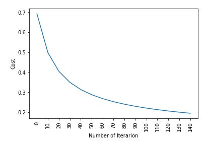
plt.plot(index, cost_list2)
plt.xticks(index, rotation ='vertical')
plt.xlabel("Number of Iterarion")
plt.ylabel("Cost")
plt.show()
return parameters, gradients, cost_list
Code : Predictions
def predict(w, b, x_test):
# x_test is a input for forward propagation
z = sigmoid(np.dot(w.T, x_test)+b)
Y_prediction = np.zeros((1, x_test.shape[1]))
# if z is bigger than 0.5, our prediction is sign one (y_head = 1),
# if z is smaller than 0.5, our prediction is sign zero (y_head = 0),
for i in range(z.shape[1]):
if z[0, i]<= 0.5:
Y_prediction[0, i] = 0
else:
Y_prediction[0, i] = 1
return Y_prediction
Code : Logistic Regression
def logistic_regression(x_train, y_train, x_test, y_test,
learning_rate, num_iterations):
dimension = x_train.shape[0]
w, b = initialize_weights_and_bias(dimension)
parameters, gradients, cost_list = update(
w, b, x_train, y_train, learning_rate, num_iterations)
y_prediction_test = predict(
parameters["weight"], parameters["bias"], x_test)
y_prediction_train = predict(
parameters["weight"], parameters["bias"], x_train)
# train / test Errors
print("train accuracy: {} %".format(
100 - np.mean(np.abs(y_prediction_train - y_train)) * 100))
print("test accuracy: {} %".format(
100 - np.mean(np.abs(y_prediction_test - y_test)) * 100))
logistic_regression(x_train, y_train, x_test,
y_test, learning_rate = 1, num_iterations = 100)
Output :
Cost after iteration 0: 0.692836
Cost after iteration 10: 0.498576
Cost after iteration 20: 0.404996
Cost after iteration 30: 0.350059
Cost after iteration 40: 0.313747
Cost after iteration 50: 0.287767
Cost after iteration 60: 0.268114
Cost after iteration 70: 0.252627
Cost after iteration 80: 0.240036
Cost after iteration 90: 0.229543
Cost after iteration 100: 0.220624
Cost after iteration 110: 0.212920
Cost after iteration 120: 0.206175
Cost after iteration 130: 0.200201
Cost after iteration 140: 0.194860
Output :
train accuracy: 37.267080745341616 %
test accuracy: 37.2093023255814 %
Code : Checking results with linear_model.LogisticRegression
from sklearn.impute import SimpleImputer
from sklearn import linear_model
# Create an imputer to replace NaN with the mean of the column
imputer = SimpleImputer(strategy='mean')
# Fit the imputer on the training data and transform both training and test data
x_train = imputer.fit_transform(x_train.T).T
x_test = imputer.transform(x_test.T).T
logreg = linear_model.LogisticRegression(random_state = 42, max_iter = 150)
print("test accuracy: {} ".format(
logreg.fit(x_train.T, y_train.T).score(x_test.T, y_test.T)))
print("train accuracy: {} ".format(
logreg.fit(x_train.T, y_train.T).score(x_train.T, y_train.T)))
# This code is modified by Susobhan Akhuli
Output :
test accuracy: 0.627906976744186
train accuracy: 0.6273291925465838
Get the complete notebook and dataset link here:
Notebook link : click here.
Dataset link : click here