When a movie is produced then the director would certainly like to maximize his/her movie’s revenue. But can we predict what will be the revenue of a movie by using its genre or budget information? This is exactly what we’ll learn in this article, we will learn how to implement a machine learning algorithm that can predict a box office revenue by using the genre of the movie and other related features.

Importing Libraries and Dataset

Python libraries make it easy for us to handle the data and perform typical and complex tasks with a single line of code.

• Pandas – This library helps to load the data frame in a 2D array format and has multiple functions to perform analysis tasks in one go.
• Numpy – Numpy arrays are very fast and can perform large computations in a very short time.
• Matplotlib/Seaborn – This library is used to draw visualizations.
• Sklearn – This module contains multiple libraries are having pre-implemented functions to perform tasks from data preprocessing to model development and evaluation.
• XGBoost – This contains the eXtreme Gradient Boosting machine learning algorithm which is one of the algorithms which helps us to achieve high accuracy on predictions.

import numpy as np
import pandas as pd
import matplotlib.pyplot as plt
import seaborn as sb
from sklearn.model_selection import train_test_split
from sklearn.preprocessing import LabelEncoder, StandardScaler
from sklearn.feature_extraction.text import CountVectorizer
from sklearn import metrics
from xgboost import XGBRegressor

import warnings
warnings.filterwarnings('ignore')

Now load the dataset into the panda’s data frame.

df = pd.read_csv('boxoffice.csv',
                 encoding='latin-1')
df.head()

Output:

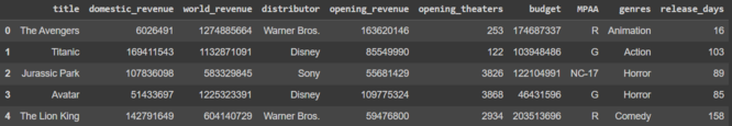
df.head()

Now let’s check the size of the dataset.

df.shape

Output:

(2694, 10)

Let’s check which column of the dataset contains which type of data.

df.info()

Output:

<class 'pandas.core.frame.DataFrame'>
RangeIndex: 2694 entries, 0 to 2693
Data columns (total 10 columns):
 #   Column            Non-Null Count  Dtype 
---  ------            --------------  ----- 
 0   title             2694 non-null   object
 1   domestic_revenue  2694 non-null   int64 
 2   world_revenue     2694 non-null   int64 
 3   distributor       2694 non-null   object
 4   opening_revenue   2694 non-null   int64 
 5   opening_theaters  2694 non-null   int64 
 6   budget            2694 non-null   int64 
 7   MPAA              2694 non-null   object
 8   genres            2694 non-null   object
 9   release_days      2694 non-null   int64 
dtypes: int64(6), object(4)
memory usage: 210.6+ KB

Here we can observe an unusual discrepancy in the dtype column the columns which should be in the number format are also in the object type. This means we need to clean the data before moving any further.

df.describe().T

Output:

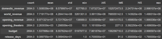
Describe

Data Cleaning

There are times when we need to clean the data because the raw data contains lots of noise and irregularities and we cannot train an ML model on such data. Hence, data cleaning is an important part of any machine-learning pipeline.

# We will be predicting only
# domestic_revenue in this article.

to_remove = ['world_revenue', 'opening_revenue']
df.drop(to_remove, axis=1, inplace=True)

Let’s check what is the percentage of entries in each column that is null.

df.isnull().sum() * 100 / df.shape[0]

Output :

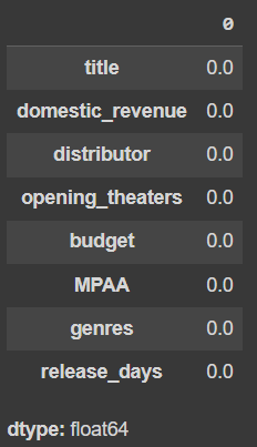
percentage of entries in each column that is null

# Handling the null value columns
df.drop('budget', axis=1, inplace=True)

for col in ['MPAA', 'genres']:
    df[col] = df[col].fillna(df[col].mode()[0])

df.dropna(inplace=True)

df.isnull().sum().sum()

Output:

0

df['domestic_revenue'] = df['domestic_revenue'].astype(str).str[1:]

for col in ['domestic_revenue', 'opening_theaters', 'release_days']:
    df[col] = df[col].astype(str).str.replace(',', '') 

    # Selecting rows with no null values 
    # in the columns on which we are iterating. 
    temp = (~df[col].isnull()) 
    df[temp][col] = df[temp][col].convert_dtypes(float) 

    df[col] = pd.to_numeric(df[col], errors='coerce')
    
# This code is modified by Susobhan Akhuli

Exploratory Data Analysis

EDA is an approach to analyzing the data using visual techniques. It is used to discover trends, and patterns, or to check assumptions with the help of statistical summaries and graphical representations. 

plt.figure(figsize=(10, 5))
sb.countplot(df['MPAA'])
plt.show()

Output:

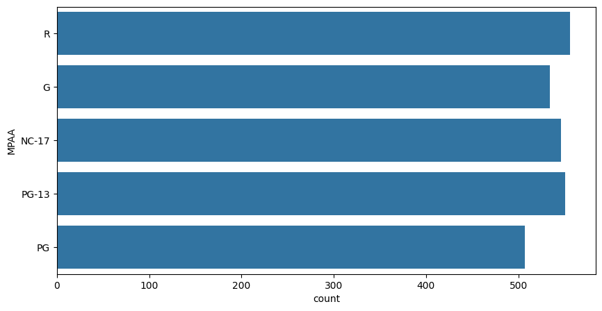
countplot

df.groupby('MPAA')['domestic_revenue'].mean()

# This code is modified by Susobhan Akhuli

Output:

MPAA    domestic_revenue
G    3.426099e+07
NC-17    3.452006e+07
PG    3.697347e+07
PG-13    3.510989e+07
R    3.670206e+07

dtype: float64

Here we can observe that the movies with PG or R ratings generally have their revenue higher than the other rating class.

plt.subplots(figsize=(15, 5))

features = ['domestic_revenue', 'opening_theaters', 'release_days']
for i, col in enumerate(features):
    plt.subplot(1, 3, i+1)
    sb.distplot(df[col])
plt.tight_layout()
plt.show()

Output:

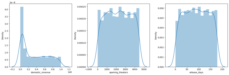
distplot

plt.subplots(figsize=(15, 5))
for i, col in enumerate(features):
    plt.subplot(1, 3, i+1)
    sb.boxplot(df[col])
plt.tight_layout()
plt.show()

Output:

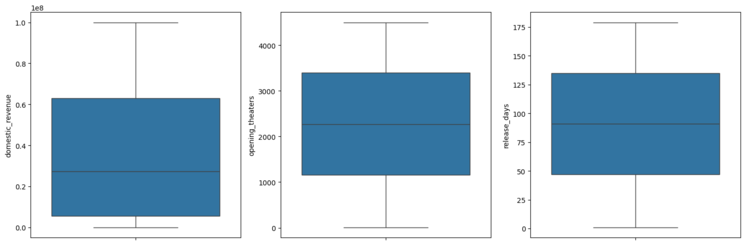
Outliers

Certainly, there are no outliers in the above features.

for col in features:
  df[col] = df[col].apply(lambda x: np.log10(x))

Now the data in the columns we have visualized above should be close to normal distribution.

plt.subplots(figsize=(15, 5))
for i, col in enumerate(features):
    plt.subplot(1, 3, i+1)
    sb.distplot(df[col])
plt.tight_layout()
plt.show()

Output:

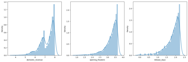
normal distribution

Creating Features from the Genre

vectorizer = CountVectorizer() 
vectorizer.fit(df['genres']) 
features = vectorizer.transform(df['genres']).toarray() 

genres = vectorizer.get_feature_names_out() 
for i, name in enumerate(genres): 
    df[name] = features[:, i] 

df.drop('genres', axis=1, inplace=True)

# This code is modified by Susobhan Akhuli

But there will be certain genres that are not that frequent which will lead to increases in the complexity of the model unnecessarily. So, we will remove those genres which are very rare.

removed = 0
# Check if 'action' and 'western' columns exist before slicing
if 'action' in df.columns and 'western' in df.columns:
    for col in df.loc[:, 'action':'western'].columns: 

        # Removing columns having more 
        # than 95% of the values as zero. 
        if (df[col] == 0).mean() > 0.95: 
            removed += 1
            df.drop(col, axis=1, inplace=True) 

print(removed) 
print(df.shape)

# This code is modified by Susobhan Akhuli

Output:

0
(2694, 12)

for col in ['distributor', 'MPAA']:
    le = LabelEncoder()
    df[col] = le.fit_transform(df[col])

As all the categorical features have been labeled encoded let’s check if there are highly correlated features in the dataset.

plt.figure(figsize=(8, 8))
sb.heatmap(df.select_dtypes(include=np.number).corr() > 0.8, 
            annot=True, 
            cbar=False) 
plt.show()

# This code is modified by Susobhan Akhuli

Output:

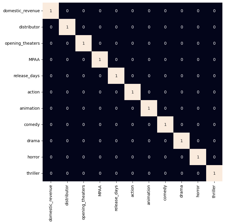
heatmap

Model Development

Now we will separate the features and target variables and split them into training and the testing data by using which we will select the model which is performing best on the validation data.

features = df.drop(['title', 'domestic_revenue'], axis=1) 
target = df['domestic_revenue'].values 

X_train, X_val, Y_train, Y_val = train_test_split(features, target, 
                                    test_size=0.1, 
                                    random_state=22) 
X_train.shape, X_val.shape 

# This code is modified by Susobhan Akhuli

Output:

((2424, 10), (270, 10))

# Normalizing the features for stable and fast training.
scaler = StandardScaler()
X_train = scaler.fit_transform(X_train)
X_val = scaler.transform(X_val)

XGBoost library models help to achieve state-of-the-art results most of the time so, we will also train this model to get better results.

from sklearn.metrics import mean_absolute_error as mae
model = XGBRegressor()
model.fit(X_train, Y_train)

We can now use the leftover validation dataset to evaluate the performance of the model.

train_preds = model.predict(X_train) 
print('Training Error : ', mae(Y_train, train_preds)) 

val_preds = model.predict(X_val) 
print('Validation Error : ', mae(Y_val, val_preds)) 
print() 

# This code is modified by Susobhan Akhuli

Output:

Training Error :  0.2104541861999253
Validation Error :  0.6358190127903746

This mean absolute error value we are looking at is between the logarithm of the predicted values and the actual values so, the actual error will be higher than what we are observing above.

Get the Complete notebook:

Notebook: click here.

Dataset : click here.