
In this article, we shall build a Stock Price Prediction project using TensorFlow. Stock Market price analysis is a Timeseries approach and can be performed using a Recurrent Neural Network. To implement this we shall Tensorflow. Tensorflow is an open-source Python framework, famously known for its Deep Learning and Machine Learning functionalities. Building Neural Networks becomes easy by writing just a few lines of Tensorflow code.
Importing Libraries and Dataset
Python libraries make it very easy for us to handle the data and perform typical and complex tasks with a single line of code.
- Pandas – This library helps to load the data frame in a 2D array format and has multiple functions to perform analysis tasks in one go.
- Numpy – Numpy arrays are very fast and can perform large computations in a very short time.
- Matplotlib/Seaborn – This library is used to draw visualizations.
- TensorFlow – This is an open-source library that is used for Machine Learning and Artificial intelligence and provides a range of functions to achieve complex functionalities with single lines of code.
import pandas as pd
import matplotlib.pyplot as plt
import numpy as np
import tensorflow as tf
from tensorflow import keras
import seaborn as sns
import os
from datetime import datetime

import warnings
warnings.filterwarnings("ignore")
Now let’s load the dataset into the pandas dataframe.
data = pd.read_csv('all_stocks_5yr.csv', delimiter=',', on_bad_lines='skip')
print(data.shape)
print(data.sample(7))

# This code is modified by Susobhan Akhuli
Output:
(619040, 7)

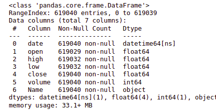
Since the given data consists of a date feature, this is more likely to be an ‘object’ data type.
data.info()
Output:

Whenever we deal with the date or time feature, it should always be in the DateTime data type. Pandas library helps us convert the object date feature to the DateTime data type.
data['date'] = pd.to_datetime(data['date'])
data.info()
Exploratory Data Analysis
EDA also known as Exploratory Data Analysis is a technique that is used to analyze the data through visualization and manipulation. For this project let us visualize the data of famous companies such as Nvidia, Google, Apple, Facebook, and so on.
First, let us consider a few companies and visualize the distribution of open and closed Stock prices through 5 years.
data['date'] = pd.to_datetime(data['date'])
# date vs open
# date vs close

# Define the list of companies you want to plot
companies = ['AAPL', 'AMD', 'FB', 'GOOGL', 'AMZN', 'NVDA', 'EBAY', 'CSCO', 'IBM']

plt.figure(figsize=(15, 8))
for index, company in enumerate(companies, 1):
    plt.subplot(3, 3, index)
    c = data[data['Name'] == company]
    plt.plot(c['date'], c['close'], c="r", label="close", marker="+")
    plt.plot(c['date'], c['open'], c="g", label="open", marker="^")
    plt.title(company)
    plt.legend()
    plt.tight_layout()

# This code is modified by Susobhan Akhuli
Output:
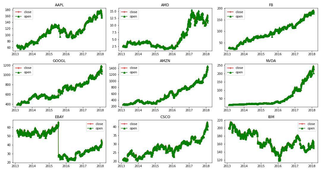
Analyzing Close and Open prices for stocks of 9 different country
Now let’s plot the volume of trade for these 9 stocks as well as a function of time.
plt.figure(figsize=(15, 8))
for index, company in enumerate(companies, 1):
    plt.subplot(3, 3, index)
    c = data[data['Name'] == company]
    plt.plot(c['date'], c['volume'], c='purple', marker='*')
    plt.title(f"{company} Volume")
    plt.tight_layout()
Output:
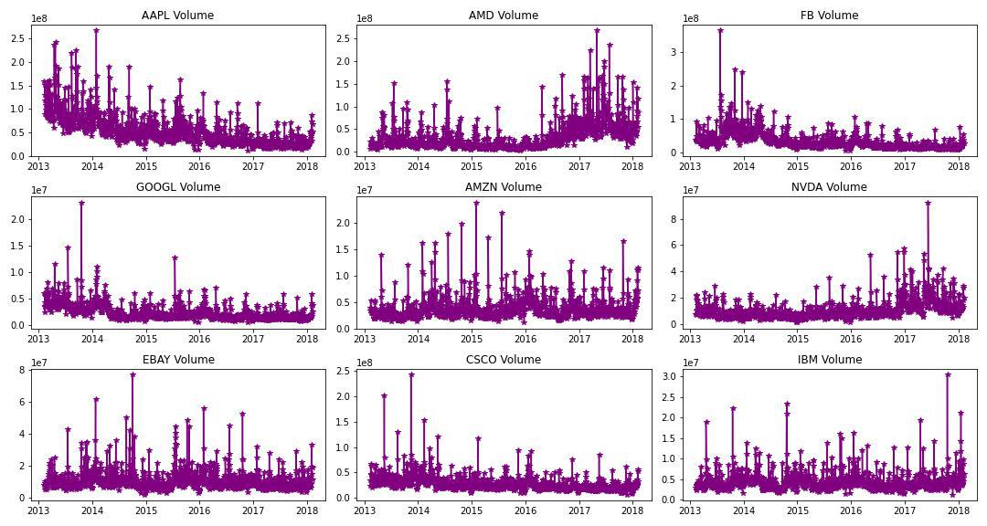
Analyzing volume for stocks of 9 different country
Now let’s analyze the data for Apple Stocks from 2013 to 2018.
apple = data[data['Name'] == 'AAPL']
prediction_range = apple.loc[(apple['date'] > datetime(2013,1,1))
 & (apple['date']<datetime(2018,1,1))]
plt.plot(apple['date'],apple['close'])
plt.xlabel("Date")
plt.ylabel("Close")
plt.title("Apple Stock Prices")
plt.show()
Output:

The overall trend in the prices of the Apple Stocks
Now let’s select a subset of the whole data as the training data so, that we will be left with a subset of the data for the validation part as well.
close_data = apple.filter(['close'])
dataset = close_data.values
training = int(np.ceil(len(dataset) * .95))
print(training)
Output:
1197
Now we have the training data length, next applying scaling and preparing features and labels that are x_train and y_train.
from sklearn.preprocessing import MinMaxScaler

scaler = MinMaxScaler(feature_range=(0, 1))
scaled_data = scaler.fit_transform(dataset)

train_data = scaled_data[0:int(training), :]
# prepare feature and labels
x_train = []
y_train = []

for i in range(60, len(train_data)):
    x_train.append(train_data[i-60:i, 0])
    y_train.append(train_data[i, 0])

x_train, y_train = np.array(x_train), np.array(y_train)
x_train = np.reshape(x_train, (x_train.shape[0], x_train.shape[1], 1))
Build Gated RNN- LSTM network using TensorFlow
Using TensorFlow, we can easily create LSTM-gated RNN cells. LSTM is used in Recurrent Neural Networks for sequence models and time series data. LSTM is used to avoid the vanishing gradient issue which is widely occurred in training RNN. To stack multiple LSTM in TensorFlow it is mandatory to use return_sequences = True. Since our data is time series varying we apply no activation to the output layer and it remains as 1 node.
model = keras.models.Sequential()
model.add(keras.layers.LSTM(units=64,
                            return_sequences=True,
                            input_shape=(x_train.shape[1], 1)))
model.add(keras.layers.LSTM(units=64))
model.add(keras.layers.Dense(32))
model.add(keras.layers.Dropout(0.5))
model.add(keras.layers.Dense(1))
model.summary
Output:
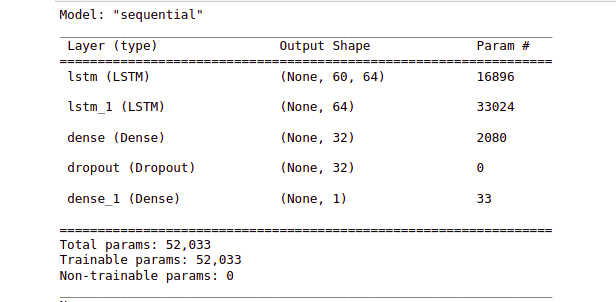
Model summary to analyze the architecture of the model
Model Compilation and Training
While compiling a model we provide these three essential parameters:
- optimizer – This is the method that helps to optimize the cost function by using gradient descent.
- loss – The loss function by which we monitor whether the model is improving with training or not.
- metrics – This helps to evaluate the model by predicting the training and the validation data.
model.compile(optimizer='adam',
              loss='mean_squared_error')
history = model.fit(x_train,
                    y_train,
                    epochs=10)
Output:
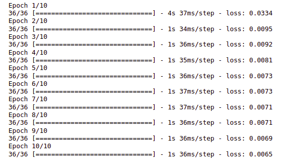
Progress of model training epoch by epoch
For predicting we require testing data, so we first create the testing data and then proceed with the model prediction.
test_data = scaled_data[training - 60:, :]
x_test = []
y_test = dataset[training:, :]
for i in range(60, len(test_data)):
    x_test.append(test_data[i-60:i, 0])

x_test = np.array(x_test)
x_test = np.reshape(x_test, (x_test.shape[0], x_test.shape[1], 1))

# predict the testing data
predictions = model.predict(x_test)
predictions = scaler.inverse_transform(predictions)

# evaluation metrics
mse = np.mean(((predictions - y_test) ** 2))
print("MSE", mse)
print("RMSE", np.sqrt(mse))
Output:
2/2 [==============================] - 1s 13ms/step
MSE 34.42497277619552
RMSE 5.867279844714714
Now that we have predicted the testing data, let us visualize the final results.
train = apple[:training]
test = apple[training:]
test['Predictions'] = predictions

plt.figure(figsize=(10, 8))
plt.plot(train['date'], train['close'])
plt.plot(test['date'], test[['close', 'Predictions']])
plt.title('Apple Stock Close Price')
plt.xlabel('Date')
plt.ylabel("Close")
plt.legend(['Train', 'Test', 'Predictions'])

# This code is modified by Susobhan Akhuli
Output:

Prediction for Stock Prices of Apple
Get the complete notebook link here
Colab Link : click here.
Dataset Link : click here.